Numerical procedure
For a crack of any shape, such as curved, we assume it can be represented with sufficient accuracy by N straight segments, joined end by end. The positions of the segments are specified with reference to the x, y co-ordinate system shown in Figure 2-2. If the surface of the crack are subjected to stress (for example, a uniform fluid pressure - p), they will displace relative to one another. The displacement discontinuity method is a means of finding a discrete approximation to the smooth distribution of relative displacement that exits in reality. The discrete approximation is found with reference to the N subdivisions of the crack depicted in Figure 2-2a. Each of the subdivisions is a boundary element and represents an elemental displacement discontinuity.
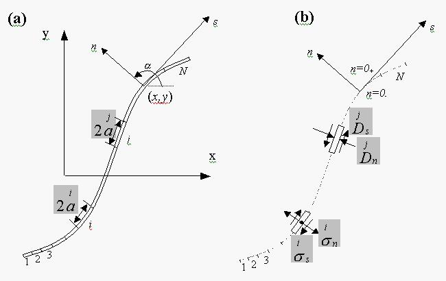
Figure 2-2. Representation of a crack by N elemental displacement discontinuities.
The elemental displacement discontinuities are defined with respect to the
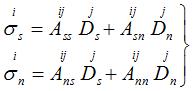
local co-ordinates s and n indicated in Figure 2-2. Figure 2-2b
depicts a single elemental displacement discontinuity at jth
segment of the crack. The components of discontinuity in the s and n
directions at this segment are donated as ![]() and
and ![]() . These
quantities are defined as follows:
. These
quantities are defined as follows:
2-5
In these definitions, ![]() and
and ![]() refer to the shear (s) and normal (n)
displacement of the jth segment of the crack.
The superscripts '+' and '-' denote the positive and negative surfaces of the
crack with respect to local co-ordinate n.
refer to the shear (s) and normal (n)
displacement of the jth segment of the crack.
The superscripts '+' and '-' denote the positive and negative surfaces of the
crack with respect to local co-ordinate n.
The local displacements ![]() and
and ![]() form the two components of a vector. They are
positive in the positive direction of s and n, irrespective of
whether we are considering the positive or negative surface of the crack. As a
consequence, it follows from Equation 2-5 that the normal component of
displacement discontinuity
form the two components of a vector. They are
positive in the positive direction of s and n, irrespective of
whether we are considering the positive or negative surface of the crack. As a
consequence, it follows from Equation 2-5 that the normal component of
displacement discontinuity ![]() is positive if the two surfaces of the crack
displace toward one another. Similarly, the shear component
is positive if the two surfaces of the crack
displace toward one another. Similarly, the shear component ![]() is positive if the
positive surface of the crack moves to the left with respect to the negative
surface.
is positive if the
positive surface of the crack moves to the left with respect to the negative
surface.
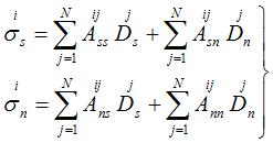
The effects of a single elemental displacement discontinuity on the displacements and stresses at an arbitrary point in the infinite solid can be computed from the results for section 2.1.1, provided we suitably transform the equations to account for the position and orientation of the line segment in question. In particular, the shear and normal stresses at the midpoint of the ith element in Figure 2-2b can be expressed in terms of the displacement discontinuity components at the jth element as follows:
 i=1 to N 2-6
where ![]() ,etc., are the boundary influence
coefficients for the stresses. The coefficient
,etc., are the boundary influence
coefficients for the stresses. The coefficient ![]() , for example, gives the
normal stress at the midpoint of the ith
element (i.e.
, for example, gives the
normal stress at the midpoint of the ith
element (i.e. ![]() ) due to a constant unit shear displacement
discontinuity over the jth element (i.e.
) due to a constant unit shear displacement
discontinuity over the jth element (i.e. ![]() =1).
=1).
Returning now to the crack problem depicted in Figure 2-2b, we place an elemental displacement discontinuity at each of the N segments along the crack and write, from Equation 2-6,
 i=1 to N 2-7
If we specify the values of the stress ![]() and
and ![]() for each element of the
crack, then Equation 2-7 is a system of 2N simultaneous linear equations
in 2N unknowns, namely the elemental displacement discontinuity
components
for each element of the
crack, then Equation 2-7 is a system of 2N simultaneous linear equations
in 2N unknowns, namely the elemental displacement discontinuity
components ![]() and
and ![]() . We can find the displacements and stresses
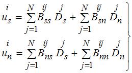
at designated points in the body by using the principle of superposition. In
particular, the displacements along the crack of Figure 2-2a are given by
expressions of the form
. We can find the displacements and stresses
at designated points in the body by using the principle of superposition. In
particular, the displacements along the crack of Figure 2-2a are given by
expressions of the form
 i=1 to N 2-8
where ![]() , etc., are the boundary influence
coefficients for the displacements. The displacements are discontinuous when
passing from one side of the jth element to
the other, so we must distinguish between these two sides when computing the
influence coefficients in Equation 2-8. The diagonal terms of the influence
coefficients in these equations have the values
, etc., are the boundary influence
coefficients for the displacements. The displacements are discontinuous when
passing from one side of the jth element to
the other, so we must distinguish between these two sides when computing the
influence coefficients in Equation 2-8. The diagonal terms of the influence
coefficients in these equations have the values
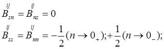 2-9
2-9
The remaining coefficients (i.e. the ones for which ij)
are continuous and they can be obtained by using Equations 2-1, 2-2 and 2-3 in
Section 2.1.1. Displacements ![]() and
and ![]() in Equation 2-8 will exhibit constant
discontinuities
in Equation 2-8 will exhibit constant
discontinuities ![]() and
and ![]() , as required.
, as required.